Finishing the Spreadsheet
To finish off the Excel spreadsheet you have been working
on in this section, we'll add figures for the weekly cost and yearly
costs of the chocolate addiction. We'll use AutoFill and SUM.
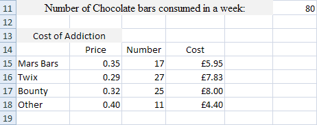
The bottom of our spreadsheet looks like this:

We now have how much each individual chocolate bar is
costing us each week. The next things to do is to add them all up to
arrive at a weekly figure for all chocolate bars.
To calculate the weekly cost of the chocolate addiction, you can use
the Excel SUM function. But there's an even easier way - use Auto Fill
and SUM. Try this.- Click inside cell F20
- Click inside the Formula bar at the top and enter = SU
- When you see the drop down list of functions, double click SUM
- Now click inside D15 of you spreadsheet
- Excel will enter the Cell for you in the formula bar:

- Notice the marching ants around Cell D15, and that there is a blue border with blue squares
- Hold your mouse over the bottom right blue square until your cursor changes to a double-headed arrow:

- Now hold your left mouse button down and drag down to cell D18
- Let go and Excel will enter the rest of the formula for you:

Press the enter key on your keyboard to finish off the
rest of the formula:

If you did that correctly, you should have a figure of
26.18 in cell F20. That's how much our chocolate bar addiction is costing
each week.
To work out how much the addiction is costing every year, we can multiply
the weekly cost of the addiction by 52 (the number of weeks in a year).
First, enter some suitable text in cell A21, something like "Annual
Cost of Chocolate addiction". The answer can then go in cell F21,
under the weekly cost.- Click into cell F21 on your spreadsheet
- Then click into the formula bar at the top
- Enter the following:
= F20 * 52
Hit the enter key on your keyboard, and the correct answer
should appear.
Cell F20 is where the weekly total is. Excel already knows
what formula is inside of this cell, so only the cell reference is needed.
After the multiply symbol, we then only need to enter the number of
weeks in a year.
The answer you should have in cell F21 is 1, 361.36. You spreadsheet
should look like ours below:
The formula we just used mixes a cell reference with a
number. Excel doesn't mind you doing it this way, just as long as there's
something to multiply. So you can do things this way:
= 26.18 * 52
Or this way:
= F20 * 52
If you have the number 52 typed into say cell H20, you could just do
this:
= F20 * H20
Add a Comment to a Cell
A comment can be added to any cell on your spreadsheet.
When you hover your mouse pointer over a cell that contains a comment,
you'll see the comment appear in a sort of Sticky-Note. To see how they
work, study the spreadsheet below:

The formula in cell B1 above gives you a random number
from 1 to 49. A new number can be had by clicking the "Calculate
Now" button on the Formula menu.
To let users know what to do, we'll add a comment to cell B1.
=RANDBETWEEN(1, 49)
The formula will generate a Random number between 1 and 49. Once you
have the above spreadsheet up and running, click inside B1 and try it
out:- From the menu bars on the Ribbon at the top of Excel, click on Formula
- Locate the Calculation panel, and then click on Calculate Now:

Excel 2007 will refresh the calculation and enter a new
random number for you. To let people know about this, you can add your
comment to the cell. To add a comment to cell B1, do the following:
- Click inside cell B1 on your spreadsheet
- From the tabs on the Ribbon at the top of Excel, click on Review
- Click on New Comment

A greenish textbox will appear to the right of cell B1,
as in the image below:

The word "user" in the image above is placed
there by Excel. This is the name of the user account that was set up
in Windows. Press the backspace on your keyboard to delete this.
To add your comment, just start typing. The size of the comment area
can be increased or decreased by moving your mouse over the white circles.
Hold down the left mouse button and drag.
When you have finished typing your comment, click on any
other cell. The comment will disappear. Notice that the cell now has
a red triangle in the top right. This indicates that it contains a comment:

If you move your mouse pointer over cell B1 the comment
will appear:

To get rid of a comment, right click the cell that contains
the comment. Then, from the menu that appears, select Delete Comment.
Review Two
You've seen a spreadsheet on chocolate addiction. The
finished version looked like this:

Time now to reveal your addiction! Create a spreadsheet
like the one above, but substitute Chocolate Addiction for something
else. Examples might be: smoking, drinking, eating out, clothes, makeup
- in fact, anything that someone might be spending too much money on.
(It doesn't have to be you doing the spending: it can be entirely made
up.)
Your spreadsheet should include the following:- Daily totals
- Individual totals
- Weekly total
- Columns for Prices
- Columns for Number and Cost
- Weekly cost
- Annual cost
You can format the spreadsheet any way you like. The colour
scheme is entirely up to you. Just make sure that your spreadsheet is
easy to follow.
No comments:
Post a Comment