Microsoft Excel 2007-2013 part-2

How to Centre Text and Numbers

You saw that by clicking inside of a cell it makes it active, so that you can make changes. We want to centre all our numbers and the text. Here's the spreadsheet we have:

So we need cells A1, A2, A3 and A4 to be active. In Excel, you can do this by highlighting the cells.

• Place your mouse over cell A1
• Your pointer should now be in the shape of a white cross
• When your pointer changes to the white cross, hold your left mouse button down and drag to cell A4
• Let go of the left mouse button when cells A1, A2, A3 and A4 are highlighted
• The image below shows what you are aiming for

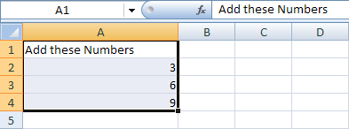
The cells highlighted in the image above have a different colour to the normal white colour of a cell. When you highlight cells, you can do things to all the cells as a group.

To centre the text and numbers in our highlighted cells, try this:

• From the Excel Ribbon at the top of the screen, locate the Alignment panel. Here's the Alignment panel in Excel 2007:

And here it is in Excel 2010 and 2013:

You can see the various alignment options laid out. These ones:

Hold your mouse over each alignment icon and you'll see an explanation of what they do. Click each icon and see what they do to your highlighted cells.

You can also click the arrow in the bottom right of the Alignment panel to bring up the Format Cells box (the one circled below).

When you click the arrow, you'll see this dialogue box:

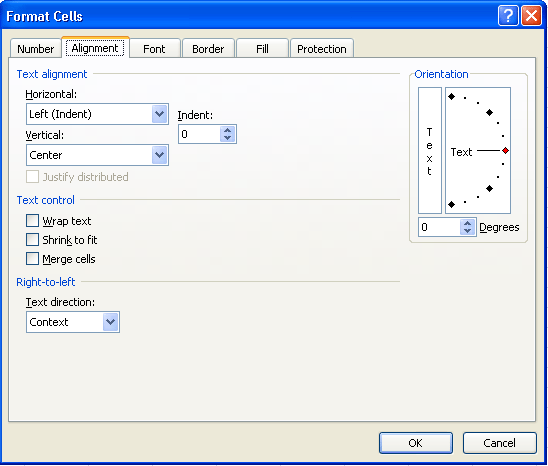
Notice the Text Alignment section at the top of the Alignment tab. It has two drop down menus, one for Horizontal alignment and one for Vertical alignment.

• Click the arrow on the Horizontal drop down menu, the one with Left (Indent) on it
• You'll see the following:

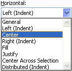
As you can see, you have plenty of options to choose from in Excel. But click on Center. Do the same for the Vertical drop down menu. Then click OK at the bottom of the Format Cells dialogue box.

The text and numbers in cells A1, A2, A3 and A4 should now be centred, and your spreadsheet will look like the one below: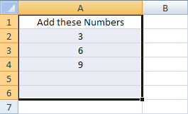

Before moving on to other types of formatting you can do in Excel, have a try of this:

• Highlight the cells A5 and A6 on your spreadsheet
• Bring up the Format Cells dialogue box, just as you did above
• Make the alignment changes from the Horizontal and Vertical drop down menus
• Click OK to get rid of the dialogue box
• Now click inside of cell A5 on your spreadsheet and enter any number you like
• Hit the Enter key

The number you just entered should also be centred. So even if a cell is empty you can still apply formatting to it.

Font Formatting

If you've been following along with the previous tutorials, you should now have a spreadsheet that looks like this:

Excel 2007 to Excel 2013 have a much wider range of formatting options than previous versions, and it's relatively easy to turn a dull spreadsheet into something that really shines. We'll start with changing the font.

Choosing a Font in Excel 2007/2013

You can pick a different font for the data you enter into cells, as well as choosing the size you want. The colour of the font, and the cell background, can be changed, too. From Excel 2007 onwards, Themes have been introduced, so that you can format your spreadsheets more easily. You'll meet these later. First, we'll see how to change the font type.

• Highlight cell A1 on your spreadsheet by simply clicking into it
• Locate the Font panel on the Excel Ribbon at the top of the page:

The font in the panel above is set to Calibri. To see more fonts, click the black down arrow:

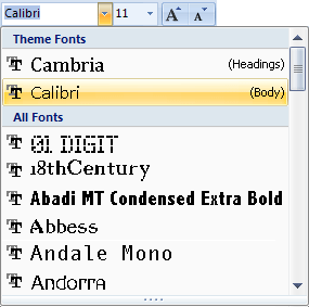
The good things about Excel 2007 and 2010/2013 is that when you move your mouse over one of the fonts on the list, the text in your selected cell (A1) will change automatically. This is just a preview, though. When you have decided on the font you want, click it with the left mouse button.

You can change the size of the font in the same way - just choose a new font size from the list of numbers in the drop down box.
If you want to change the font via the Format Cells dialogue box, as you did in previous versions of Excel, you can click the small arrow in the bottom right of the Font panel (the one circled below):

When you click the arrow, you'll see the Format Cells dialogue box. You can choose various options from this dialogue box: Font size, style, size, etc. The dialogue box looks like this:

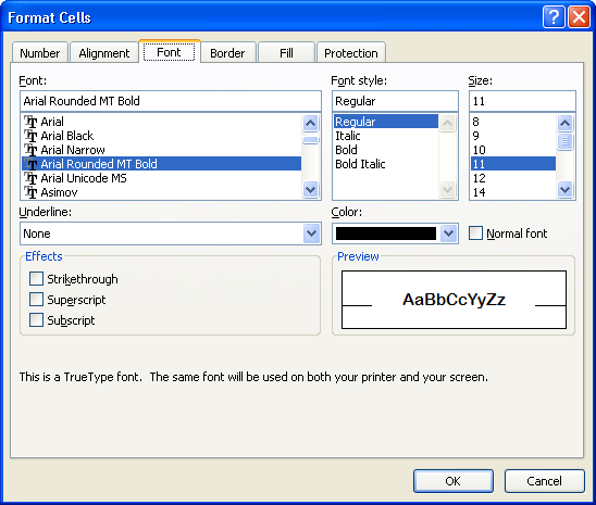
You can also set the font colour from here, and add text effects. Click OK when you have made your choices.

When you have changed the font and font size, your A1 cell might look something like this: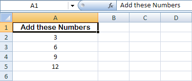

How to Change the Colour of a Cell

In the previous lesson, you saw how to change the font and font size in Excel. In this lesson, we'll look at how to change the colour of a cell.

Change the Background Colour of a Cell

To change the background colour of cells, you first have to highlight the ones you want to alter. We'll start with the cells A2 to A5. So highlight these cells on your spreadsheet.

• With the cells A2 to A5 highlighted, locate the Font panel on the Ribbon at the top of the Excel: (The image below is from Excel 2007. Later versions are the same but less colourful!)

• Locate the Paint Bucket, and click the arrow just to the right of it. You'll see some colours appear:

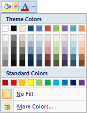
Move your mouse over any of the colours and the cells will change automatically. You can then see what the new colour looks like. Click with the left mouse button to set the colour you want. If you don't like any of the colours displayed, click on "More Colors".

Once you have the number cells formatted in a different colour, click on the cell A1. Now do exactly the same thing, only this time choose a contrasting colour for the background of this cell. Your spreadsheet should then look something like the one below.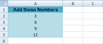

Change the Text colour

To change the colour of the text itself, click the down arrow just to the right of the letter A, which is just to the right of the Paint Bucket on the Font panel.

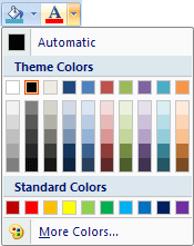
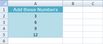
Select a colour just like you did for the background colour of the cell. Here's what your spreadsheet might look like with the background cell colour changes, and the text colour: