Microsoft Excel 2007-2013 part-3

How to save your work in Excel

Now that your spreadsheet is coming along nicely, you'll want to save your work. To save your spreadsheet, do the following.

• If you have Excel 2007, click the round Office button in the very top left of Excel 2007. This one:

When you click the Office button, you'll see the options list appear:

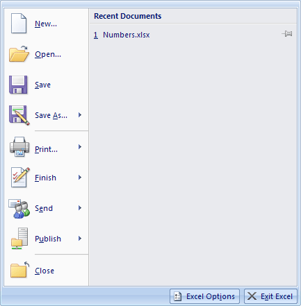
The Office button used to be a file menu in previous versions of Excel. In Excel 2007, you perform all the File operations by clicking the round Office button. Clicking Close, for example, will close the current Excel spreadsheet, but won't close down Excel itself. To close down Excel, click the "Exit Excel" button in the bottom right of this dialogue box. If you want to open a recent Excel document, click its name under the Recent Documents heading.

For Excel 2010 and 2013 users, you don't have a round Office button. Click the File tab instead to see the menu options as above: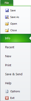

In Excel 2013, your spreadsheet will disappear when you click File and you'll see this screen:

To save your work, click the Save option in all versions. Excel 2013 users will stay on the screen above.
Under Save As in Excel 2013, you'll see three options: SkyDrive, Computer, and Add a Place. The first option is SkyDrive. This saves it to servers operated and controlled by Microsoft. This is very useful if you want to work on your Excel document from other locations. For example, you may be working on a spreadsheet in your office. Saving it to SkyDrive means you'll also be able to open it when you get home from work. When you click the SkyDrive option you'll be able to Sign In, Sign Up, or simply Learn More. We'll be saving to the Computer, though, so click this option. Then click the Browse option:

You'll then see a dialogue box like this one: (Excel 2007 and 2010 users will see this straightaway.)

In the image above, we're saving our Excel spreadsheet to a New Folder we've created in the Libraries > Documents folder.

If you have Windows XP, you'll see this at the top of your dialogue box:

Save in means "Where would you like to save your spreadsheet?" In the image above, we're saving it to a folder called excel.

Notice the blue down-pointing arrow on the Save in drop down list. Click the arrow to reveal more locations:

Choose a new location from the list, if you prefer. The large white rectangle on the Save as dialogue box will then show you all the files already in the location.

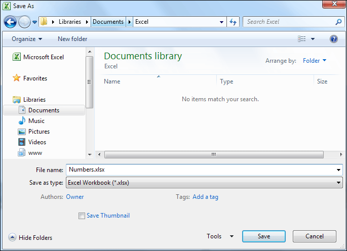
When you're happy with your file location, type a name for your file in the area at the bottom of the dialogue box :

Notice the "Save as Type" box below the file name. The type is a XLSX file, and this is new from Excel 2007. The old ending was XLS. Excel 2007 and 2010 can open older XLS files, but previous versions of Excel can't open XLSX files.)

Remember to save you work on a regular basis, by clicking either the round Office button in Excel 2007 or the File menu in Excel 2010/2013. Then click the Save option. A quicker way is to just click the disk icon on the Quick Access Toolbar in the top left of Excel (all versions):

Coming up shortly is a Review, so that you can test your new knowledge of Excel. First though, you'll need to know about currency options.

Currency Symbols in Excel

Take a look at the following spreadsheet, which you'll shortly be creating:

The C column has a heading of "Price Each". The prices all have the currency symbol. To insert the currency symbol, do this:

• Enter some prices on a spreadsheet (any will do), and highlight the cells
• With the cells highlighted, locate the Number panel on the Excel 2007 to 2013 Ribbon bar (on the Home Tab):

Click the drop down list that says General. You'll then be presented with a list of options:

Click the Currency item to add a pound sign. But if you're not in the UK, you'll see the default currency for your country.

To see other currencies, click on More (or More Number Formats in Excel 2013).The Format Cells dialogue box appears. In the Category list, click on Currency. Select a Currency sign from the Symbol list. The dialogue box will then look like this:

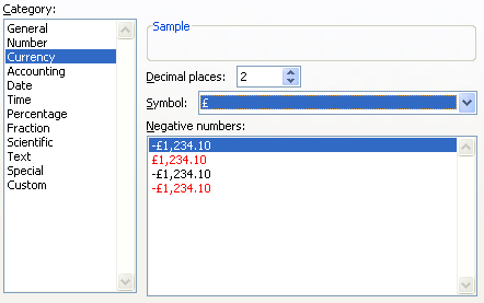
Click OK to set the pound sign as the currency.

How to Merge Cells

Study the spreadsheet below:

If you look at Row 1, you'll see that the "Shopping Bill" heading stretches across three cells. This is not three separate cells, with a colour change for each individual cell. The A1, B1 and C1 cells were merged. To merge cells, do the following.

• Type the words Shopping Bill into cell A1 of a spreadsheet
• Highlight the cells A1, B1 and C1
• On the Alignment panel of the Excel Ribbon, locate the "Merge and Center" item:

• Click the down arrow to see the following options:

Click on "Merge and Center". Your three cells will then become one - A1, to be exact!

Review One

Reproduce the simple spreadsheet below, from a junk-food addict! You can pick your own colours for the cells and data, but try to include everything that's in the image.

As well as centred text and numbers, you need to widen the columns. To get the currency symbol, see a previous section. Also in a previous section, you can see how to merge cells for the "Shopping Bill" heading. This should be one cell, and not three.

When you have produced the same spreadsheet as ours, you can move on to the next section, which is all about basic formulas in Excel.